This is a long overdue blog post on Reinforcement Learning (RL). RL is hot! You may have noticed that computers can now automatically learn to play ATARI games (from raw game pixels!), they are beating world champions at Go, simulated quadrupeds are learning to run and leap, and robots are learning how to perform complex manipulation tasks that defy explicit programming. It turns out that all of these advances fall under the umbrella of RL research. I also became interested in RL myself over the last ~year: I worked through Richard Sutton’s book, read through David Silver’s course, watched John Schulmann’s lectures, wrote an RL library in Javascript, over the summer interned at DeepMind working in the DeepRL group, and most recently pitched in a little with the design/development of OpenAI Gym, a new RL benchmarking toolkit. So I’ve certainly been on this funwagon for at least a year but until now I haven’t gotten around to writing up a short post on why RL is a big deal, what it’s about, how it all developed and where it might be going.
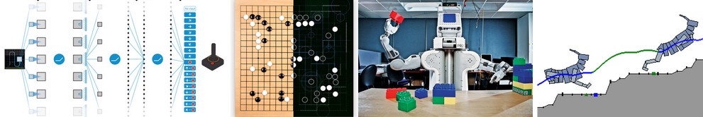
Examples of RL in the wild. From left to right: Deep Q Learning network playing ATARI, AlphaGo, Berkeley robot stacking Legos, physically-simulated quadruped leaping over terrain.
It’s interesting to reflect on the nature of recent progress in RL. I broadly like to think about four separate factors that hold back AI:
Similar to what happened in Computer Vision, the progress in RL is not driven as much as you might reasonably assume by new amazing ideas. In Computer Vision, the 2012 AlexNet was mostly a scaled up (deeper and wider) version of 1990’s ConvNets. Similarly, the ATARI Deep Q Learning paper from 2013 is an implementation of a standard algorithm (Q Learning with function approximation, which you can find in the standard RL book of Sutton 1998), where the function approximator happened to be a ConvNet. AlphaGo uses policy gradients with Monte Carlo Tree Search (MCTS) - these are also standard components. Of course, it takes a lot of skill and patience to get it to work, and multiple clever tweaks on top of old algorithms have been developed, but to a first-order approximation the main driver of recent progress is not the algorithms but (similar to Computer Vision) compute/data/infrastructure.
Now back to RL. Whenever there is a disconnect between how magical something seems and how simple it is under the hood I get all antsy and really want to write a blog post. In this case I’ve seen many people who can’t believe that we can automatically learn to play most ATARI games at human level, with one algorithm, from pixels, and from scratch - and it is amazing, and I’ve been there myself! But at the core the approach we use is also really quite profoundly dumb (though I understand it’s easy to make such claims in retrospect). Anyway, I’d like to walk you through Policy Gradients (PG), our favorite default choice for attacking RL problems at the moment. If you’re from outside of RL you might be curious why I’m not presenting DQN instead, which is an alternative and better-known RL algorithm, widely popularized by the ATARI game playing paper. It turns out that Q-Learning is not a great algorithm (you could say that DQN is so 2013 (okay I’m 50% joking)). In fact most people prefer to use Policy Gradients, including the authors of the original DQN paper who have shown Policy Gradients to work better than Q Learning when tuned well. PG is preferred because it is end-to-end: there’s an explicit policy and a principled approach that directly optimizes the expected reward. Anyway, as a running example we’ll learn to play an ATARI game (Pong!) with PG, from scratch, from pixels, with a deep neural network, and the whole thing is 130 lines of Python only using numpy as a dependency (Gist link). Lets get to it.
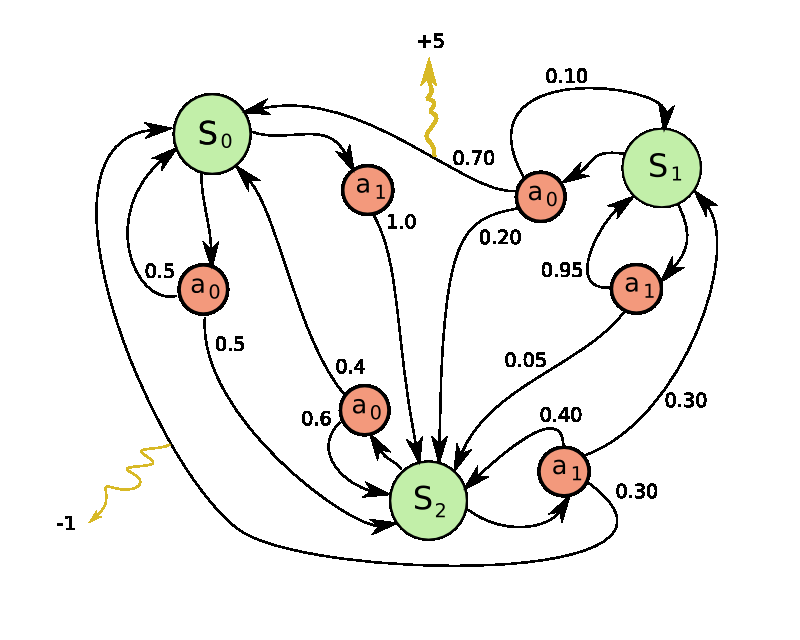
Left: The game of Pong. Right: Pong is a special case of a Markov Decision Process (MDP): A graph where each node is a particular game state and each edge is a possible (in general probabilistic) transition. Each edge also gives a reward, and the goal is to compute the optimal way of acting in any state to maximize rewards.
The game of Pong is an excellent example of a simple RL task. In the ATARI 2600 version we’ll use you play as one of the paddles (the other is controlled by a decent AI) and you have to bounce the ball past the other player (I don’t really have to explain Pong, right?). On the low level the game works as follows: we receive an image frame (a 210x160x3 byte array (integers from 0 to 255 giving pixel values)) and we get to decide if we want to move the paddle UP or DOWN (i.e. a binary choice). After every single choice the game simulator executes the action and gives us a reward: Either a +1 reward if the ball went past the opponent, a -1 reward if we missed the ball, or 0 otherwise. And of course, our goal is to move the paddle so that we get lots of reward.
As we go through the solution keep in mind that we’ll try to make very few assumptions about Pong because we secretly don’t really care about Pong; We care about complex, high-dimensional problems like robot manipulation, assembly and navigation. Pong is just a fun toy test case, something we play with while we figure out how to write very general AI systems that can one day do arbitrary useful tasks.
Policy network. First, we’re going to define a policy network that implements our player (or “agent”). This network will take the state of the game and decide what we should do (move UP or DOWN). As our favorite simple block of compute we’ll use a 2-layer neural network that takes the raw image pixels (100,800 numbers total (2101603)), and produces a single number indicating the probability of going UP. Note that it is standard to use a stochastic policy, meaning that we only produce a probability of moving UP. Every iteration we will sample from this distribution (i.e. toss a biased coin) to get the actual move. The reason for this will become more clear once we talk about training.
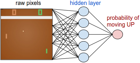
Our policy network is a 2-layer fully-connected net.
and to make things concrete here is how you might implement this policy network in Python/numpy. Suppose we’re given a vector x that holds the (preprocessed) pixel information. We would compute: